R - plotly - combine bubble and chorpleth map

Question

I would like to combine two types of maps within one map in plotly, namely bubble and choropleth map. The objective is to show population size on a country level (choropleth) as well as on a city level (bubble) by hovering with the mouse over the map.

The plotly example code for a choropleth map is as follows:

library(plotly)
    df <- read.csv('https://raw.githubusercontent.com/plotly/datasets/master/2014_world_gdp_with_codes.csv')

    # light grey boundaries
    l <- list(color = toRGB("grey"), width = 0.5)

    # specify map projection/options
    g <- list(
      showframe = FALSE,
      showcoastlines = FALSE,
      projection = list(type = 'Mercator')
    )

    plot_ly(df, z = GDP..BILLIONS., text = COUNTRY, locations = CODE, type = 'choropleth',
            color = GDP..BILLIONS., colors = 'Blues', marker = list(line = l),
            colorbar = list(tickprefix = '$', title = 'GDP Billions US$'),
            filename="r-docs/world-choropleth") %>%
      layout(title = '2014 Global GDP<br>Source:<a href="https://www.cia.gov/library/publications/the-world-factbook/fields/2195.html">CIA World Factbook</a>',
             geo = g)

The plotly example code for a bubble map is as follows:

library(plotly)
    df <- read.csv('https://raw.githubusercontent.com/plotly/datasets/master/2014_us_cities.csv')
    df$hover <- paste(df$name, "Population", df$pop/1e6, " million")

    df$q <- with(df, cut(pop, quantile(pop)))
    levels(df$q) <- paste(c("1st", "2nd", "3rd", "4th", "5th"), "Quantile")
    df$q <- as.ordered(df$q)

    g <- list(
      scope = 'usa',
      projection = list(type = 'albers usa'),
      showland = TRUE,
      landcolor = toRGB("gray85"),
      subunitwidth = 1,
      countrywidth = 1,
      subunitcolor = toRGB("white"),
      countrycolor = toRGB("white")
    )

    plot_ly(df, lon = lon, lat = lat, text = hover,
            marker = list(size = sqrt(pop/10000) + 1),
            color = q, type = 'scattergeo', locationmode = 'USA-states',
            filename="r-docs/bubble-map") %>%
      layout(title = '2014 US city populations<br>(Click legend to toggle)', geo = g)

How could one possibly merge the two types of maps into one?

Answer 1

Great question! Here's a simple example. Note:

• Use add_trace to add another chart type layer on top of the plot
• the layout of the plot is shared across all traces. layout keys describe things like the map's scope, axes, title, etc. See more layout keys.

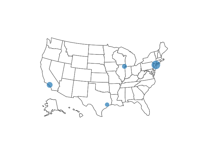
Simple bubble chart map

lon = c(-73.9865812, -118.2427266, -87.6244212, -95.3676974)
pop = c(8287238, 3826423, 2705627, 2129784)
df_cities = data.frame(cities, lat, lon, pop)

plot_ly(df_cities, lon=lon, lat=lat, 
        text=paste0(df_cities$cities,'<br>Population: ', df_cities$pop),
        marker= list(size = sqrt(pop/10000) + 1), type="scattergeo",
        filename="stackoverflow/simple-scattergeo") %>%
  layout(geo = list(scope="usa"))

Interactive version

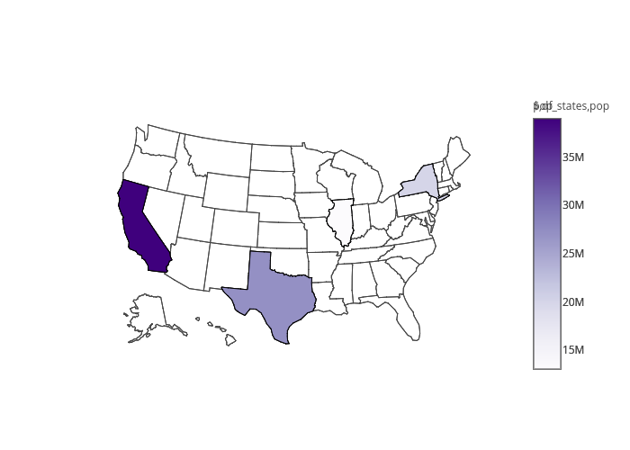
Simple choropleth chart

state_codes = c("NY", "CA", "IL", "TX")
pop = c(19746227.0, 38802500.0, 12880580.0, 26956958.0)
df_states = data.frame(state_codes, pop)

plot_ly(df_states, z=pop, locations=state_codes, text=paste0(df_states$state_codes, '<br>Population: ', df_states$pop), 
        type="choropleth", locationmode="USA-states", colors = 'Purples', filename="stackoverflow/simple-choropleth") %>%
  layout(geo = list(scope="usa"))

Interactive version

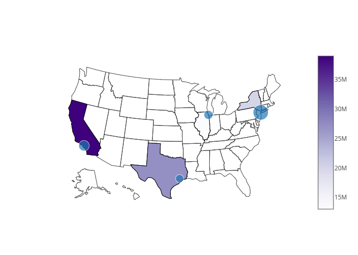
Combined choropleth and bubble chart

plot_ly(df_cities, lon=lon, lat=lat, 
        text=paste0(df_cities$cities,'<br>Population: ', df_cities$pop), 
        marker= list(size = sqrt(pop/10000) + 1), type="scattergeo",
        filename="stackoverflow/choropleth+scattergeo") %>%
  add_trace(z=df_states$pop,
            locations=df_states$state_codes, 
            text=paste0(df_states$state_codes, '<br>Population: ', df_states$pop),
            type="choropleth", 
            colors = 'Purples', 
            locationmode="USA-states") %>%
  layout(geo = list(scope="usa"))

Interactive version with hover text

Note that z and locations columns in the second trace are explicitly from the df_states dataframe. If they were from the same dataframe as the first trace (df_cities declared in plot_ly) then we could've just written z=state_codes instead of z=df_states$state_codes (as in the second example).